回归系数图
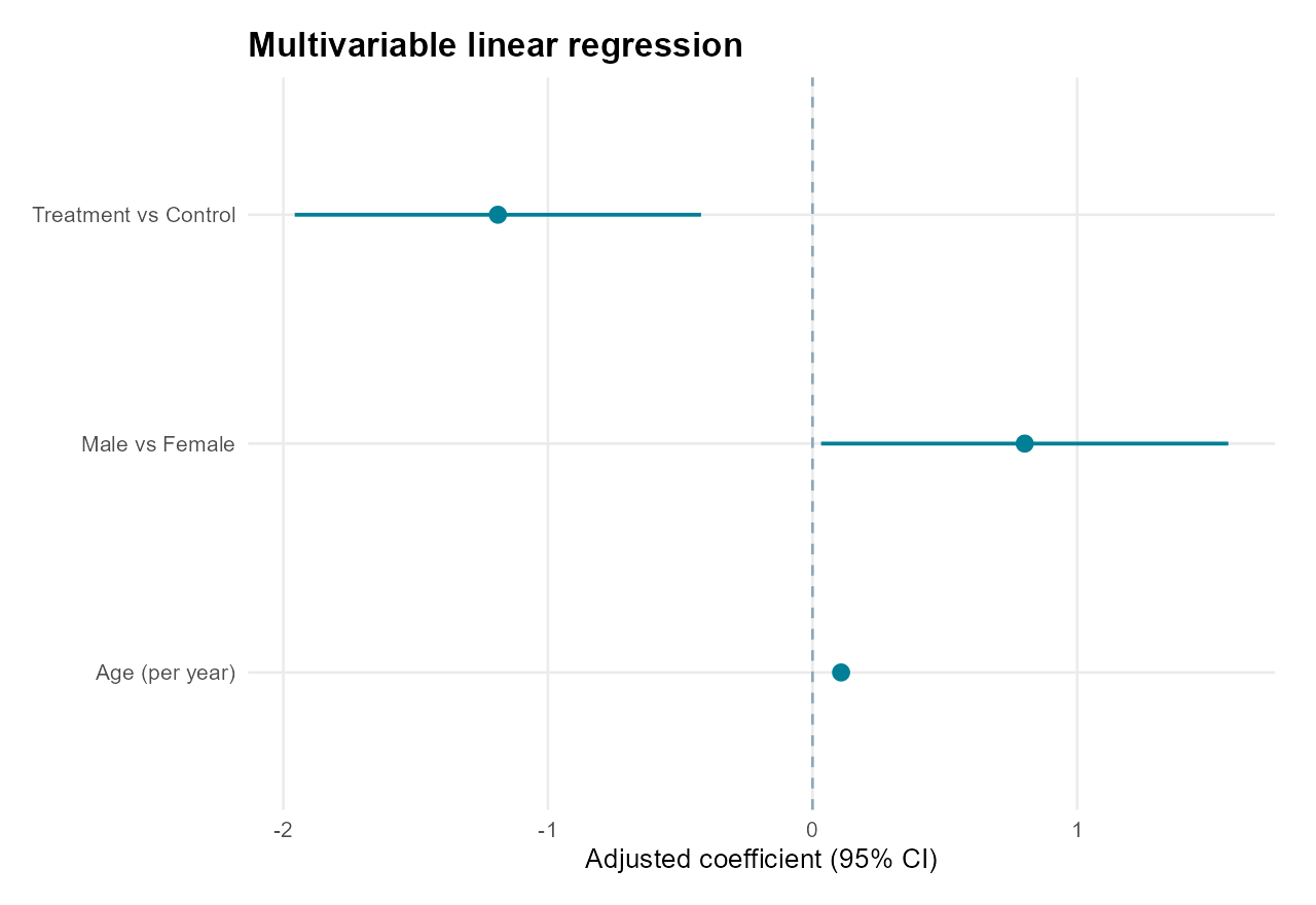
展示多变量线性模型的调整后系数与区间。
准备怎样的数据?
每行一位独立受试者。
输入字段:id、age、sex、group、value
完整 R 代码
所需包:ggplot2、jsonlite。首次使用时,先运行代码注释中的安装命令。
# 回归系数图:多变量线性回归系数及 95% CI
# 项目原创脚本,MIT 许可;模拟数据 CC0-1.0;图形 CC BY 4.0。
# 在全新 R 会话运行。每次运行会更新下方 output_dir 中的本示例文件。
# 图形标签使用英文以避免不同电脑缺少中文字体;可在参数和 labs() 中修改。

# 1. 依赖:首次使用时手动运行以下安装命令,脚本不会自动安装。
# install.packages(c("ggplot2", "jsonlite"))
required_packages <- c("ggplot2", "jsonlite")
missing_packages <- required_packages[!vapply(required_packages, requireNamespace, logical(1), quietly = TRUE)]
if (length(missing_packages)) stop("Please install: ", paste(missing_packages, collapse = ", "))
library(ggplot2)

# 2. 可修改参数:颜色、字体、导出尺寸和路径。输出路径相对于当前工作目录。
set.seed(20261014)
colors <- c("#007F96", "#B66A46")
font_family <- "sans"
figure_width <- 8
figure_height <- 5.5
output_dir <- file.path(getwd(), "rfig-regression-output")
dir.create(output_dir, recursive = TRUE, showWarnings = FALSE)
theme_set(theme_minimal(base_size = 12, base_family = font_family) +
 theme(plot.background = element_rect(fill = "white", color = NA), panel.grid.minor = element_blank(),
       plot.title = element_text(face = "bold", size = 15), legend.position = "bottom",
       plot.margin = margin(14, 18, 14, 14)))

# 3. 示例数据:每行一位独立受试者。 替换结局和模型变量,明确分类参考组、连续变量单位与调整变量。
# 使用自己的 CSV 时,将以下数据生成段替换为:
# data <- read.csv("your-data.csv", stringsAsFactors = FALSE)
# 再按本例要求设置分类顺序、检查字段、单位及缺失值。
data <- data.frame(id = 1:160, age = runif(160, 30, 75),
 sex = factor(rep(c("Female", "Male"), 80), levels = c("Female", "Male")),
 group = factor(sample(rep(c("Control", "Treatment"), each = 80)), levels = c("Control", "Treatment")))
data$value <- 8 + .08 * data$age + (data$sex == "Male") - 1.5 * (data$group == "Treatment") + rnorm(160, 0, 2.5)
stopifnot(!anyNA(data))

# 4. 统计计算与绘图。普通最小二乘模型 value ~ group + age + sex;显示非截距系数与基于 t 分布的 95% CI。年龄系数按每增加 1 岁解释,其他系数按参考组解释。无效线为 0,不能比较不同单位系数大小判断变量重要性;需检查模型假设。
model <- lm(value ~ group + age + sex, data = data)
ci <- confint(model, level = .95)[-1, , drop = FALSE]
effects <- data.frame(term = c("Treatment vs Control", "Age (per year)", "Male vs Female"), estimate = unname(coef(model)[-1]), lower = ci[,1], upper = ci[,2])
p <- ggplot(effects, aes(estimate, term)) + geom_vline(xintercept = 0, linetype = "dashed", color = "#8DA5B6") +
 geom_segment(aes(x = lower, xend = upper, yend = term), color = colors[1], linewidth = .8) + geom_point(color = colors[1], size = 3) +
 labs(x = "Adjusted coefficient (95% CI)", y = NULL, title = "Multivariable linear regression")
metrics <- list(estimate = effects$estimate, lower = effects$lower, upper = effects$upper)
print(p)

# 5. 导出:CSV 与绘图所用 data 完全一致,preview 与科研图片均来自同一个 p。
write.csv(data, file.path(output_dir, "data.csv"), row.names = FALSE, fileEncoding = "UTF-8")
ggsave(file.path(output_dir, "preview.png"), p, width = figure_width, height = figure_height, dpi = 160, bg = "white")
ggsave(file.path(output_dir, "figure.png"), p, width = figure_width, height = figure_height, dpi = 300, bg = "white")
ggsave(file.path(output_dir, "figure.pdf"), p, width = figure_width, height = figure_height, device = grDevices::pdf, bg = "white")
ggsave(file.path(output_dir, "figure.tiff"), p, width = figure_width, height = figure_height, dpi = 300, compression = "lzw", bg = "white")
jsonlite::write_json(metrics, file.path(output_dir, "metrics.json"), auto_unbox = TRUE, digits = 16, pretty = TRUE)
运行与修改
- 安装 R 和 RStudio,复制完整代码到新的 R 脚本文件,或打开下载的 .R 文件。
- 首次使用时,运行脚本顶部注释中的
install.packages()命令。 - 运行整个脚本。演示数据已包含在代码中,无需先下载 CSV。
- 图片和 CSV 保存在当前工作目录的
rfig-regression-output子目录。再次运行会更新其中的同名示例文件。
替换自己的数据
替换结局和模型变量,明确分类参考组、连续变量单位与调整变量。
将脚本“示例数据”段替换为 data <- read.csv("your-data.csv", stringsAsFactors = FALSE),再按数据字典检查列名、类型、分类顺序及单位。演示 CSV 可用作结构参考。
调整外观与导出
在参数段修改颜色、字体、图片宽高和输出目录;在 labs() 中修改标题和轴标签。脚本提供 PDF、300 dpi PNG 和 LZW 压缩 TIFF 导出。演示图使用英文标签以减少字体依赖。
数据字典
下载示例 CSV每行一位独立受试者。 演示数据不含缺失值,使用固定种子 20261014。
| 列名 | 类型 | 单位 | 含义 | 角色 |
|---|---|---|---|---|
id | 整数 | 无 | 受试者编号 | 标识 |
age | 数值 | 岁 | 年龄 | 协变量 |
sex | 分类 | 无 | Female 为参考组 | 协变量 |
group | 分类 | 无 | Control 为参考组 | 协变量 |
value | 数值 | 演示单位 | 连续结局 | Y |
统计说明与适用限制
普通最小二乘模型 value ~ group + age + sex;显示非截距系数与基于 t 分布的 95% CI。年龄系数按每增加 1 岁解释,其他系数按参考组解释。无效线为 0,不能比较不同单位系数大小判断变量重要性;需检查模型假设。
本例用于展示绘图方法。应用于真实研究前,请结合研究设计、数据质量和模型假设选择统计方法。